Documentation

Installation

• Install the latest Java Runtime Environment (Java 11 or later)
• Download the telometer app jar file. You can download using your browser, or just open a command prompt and run:

curl -k https://demarzolab.pathology.jhmi.edu/telometer/downloads/telometer-3.1.0.jar -o telometer-3.1.0.jar

• Move the jar to any directory. The data directory for Telometer is stored in the same location as where Java is executed from.

Running

• Double click jar file to start.
  If this doesn't work or you're running on a MAC, open a command prompt and run:

java -jar telometer-3.1.0.jar

Scoring

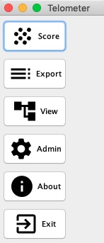
1. When Telometer starts up click the Score Button screenshot when telometer starts
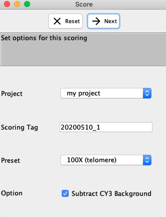
2. Fill out the options for Telometer screenshot of scoring options
   1. Project All scoring are put into 1 and only 1 project. Go to Admin if you want to add or edit existing projects.
   2. Scoring Tag: A unique identifier for this scoring. This can be anything you choose.
   3. Preset: Select the appropriate preset (usually named by the magnification) corresponding to that used when collecting the images. Selections here result in changes in the various presets
      (such as minimum and maximum spot size, rolling ball size, etc ) to values optimized for images taken at that particular magnification. Note that these presets usually work well, but were originally selected for optimal use with our own particular microscope/camera combination. Different set-ups may require adjustments of the presets for optimal performance, even if the objective magnification is the same value.
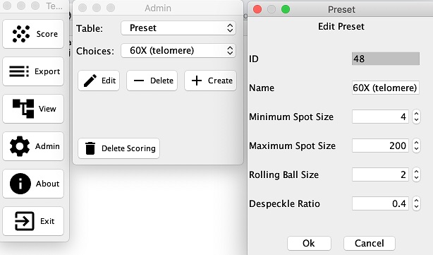
      You may add additional or edit existing presets in the Admin section. Edit Preset Screenshot
   4. Subtract Cy Noise: If this option is selected then during the final stage of analysis, the nuclear CY3 background noise is subtracted from each pixel of that cell’s telomeres. The background noise is the average intensity of all non-telomeric nuclear pixels in a cell. This option is only available to change at the beginning of analysis.
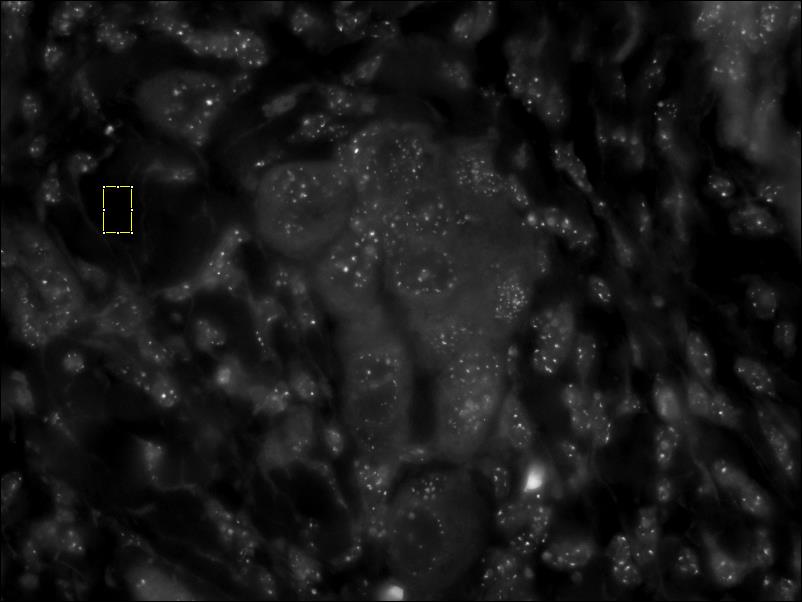
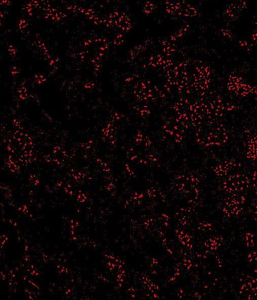
3. Select the CY3 image (the one with the FISH signals)
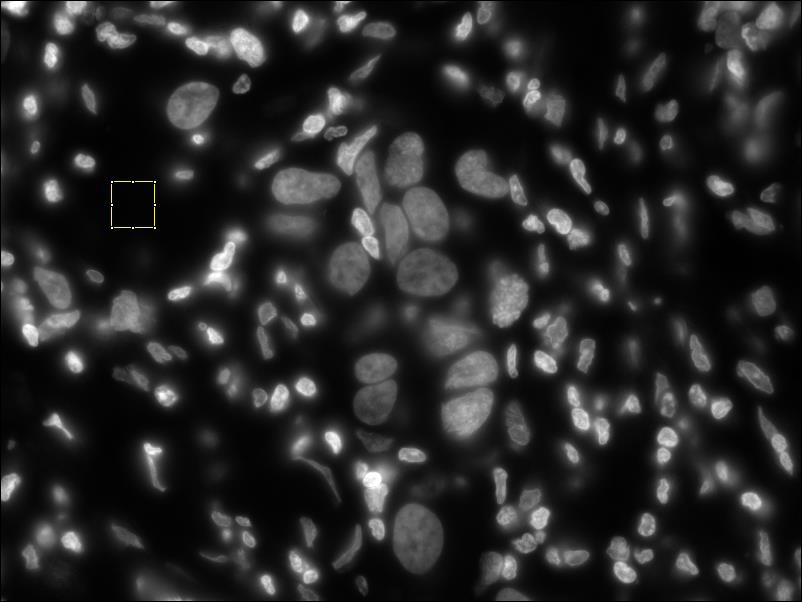
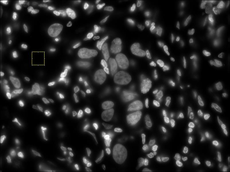
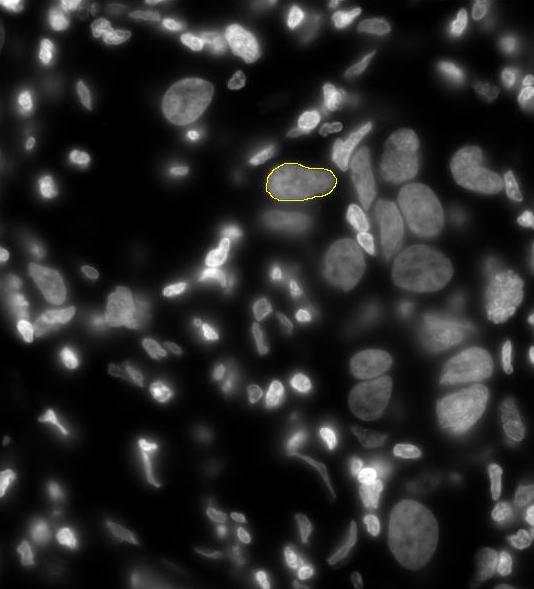
4. Select the DAPI image – the one with images of the cell nuclei (we use the DNA-binding dye DAPI for this purpose).
5. Normalize the CY3 image – Select an area of the of the CY3 image that is devoid of features and press the Next button. In some cases the changes in intensity may not be apparent. screenshot before normalizing cy3 // screenshot after normalizing cy3
6. Normalize the DAPI image (same process as CY3 image) screenshot before normalizing dapi // screenshot after normalizing dapi
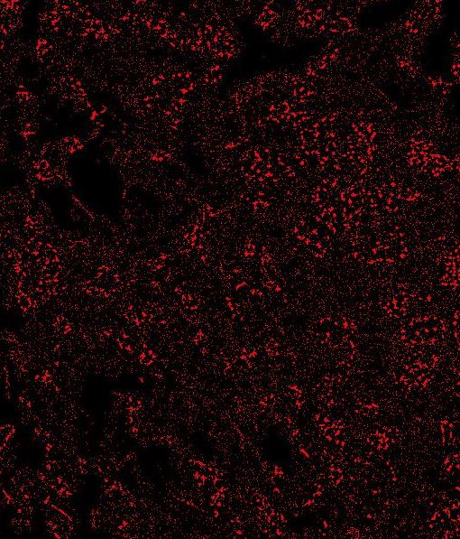
7. Segmentation of FISH objects/“Rolling Ball Background subtration” This stage will make a bitmask from the objects in the CY3 image. The first step is to run a rolling ball “background subtractor”. The rolling ball radius is automatically selected from the preset mode you have chosen. It can be changed manually as well. “Implements a rolling-ball algorithm for the removal of smooth continuous background from a two-dimensional gel image. It rolls the ball (actually a square patch on the top of a sphere) on a low-resolution (by a factor of ‘shrinkfactor’ times) copy of the original image in order to increase speed with little loss in accuracy. It uses interpolation and extrapolation to blow the shrunk image to full size.” –Description of the Rolling Ball algorithm from the ImageJ source code screenshot before ‘rolling ball’ // screenshot after ‘rolling ball’
8. Manual thresholding. Use the slider to adjust the threshold.
   1. The goal of thresholding is to find a level that maximizes the size of the spots but does not introduce too much noise. A small amount of noise is OK as this will be automatically removed. too much noise // too little noise // just right
   2. Click the Next button
   3. A despeckle filter will automatically be run immediately after the thresholding operation and will clean up most of the leftover noise. This despeckle filter counts the number of white pixels that are immediate neighbors to an origin pixel. If the number of positive pixels / 8 is greater than the despeckle ratio specified by the preset mode then the pixel will be white in the resultant image. This operation is run on every pixel in the image and depending on the despeckle ratio will reduce the amount of “salt and pepper” noise in the image and will make solid positive areas slightly larger, both effects are desirable for the next stage. NOTE: if you do adjust the Threshold, you should use the same value for each image you process in the same image set.
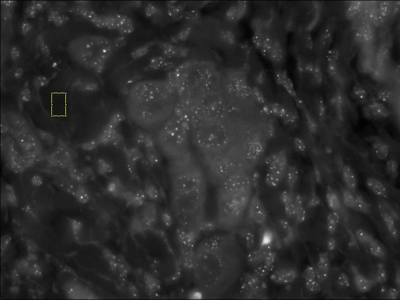
9. Selecting Nuclei for Analysis – This stage will have the user determine, by hand, which nuclei will be analyzed. Selecting a Nucleus Screenshot
   1. Draw a freehand ROI around a nucleus of interest in the DAPI image. When outlining the nuclei, draw the outline closely to the DAPI stained nuclear outline, avoiding dark pixels outside of the nucleus as much as possible. Inclusion of too much black pixel area at this stage can impact the calculated average nuclear Cy3 noise level.
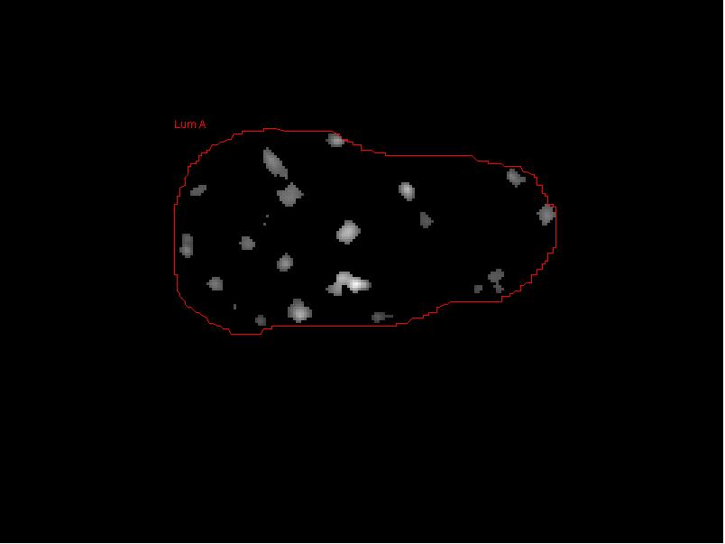
   2. In the relevants textfields, enter the cell name and choose the tissue, lesion, and cell types either by selecting from a drop down. Note that more options for these drop-down choices can be added in Admin.
   3. Click the the “Add Nucleus”" button to add this nucleus to the list of nuclei to be analyzed, Once a nucleus is selected it will be circled and labeled in red with the cell name provided. Repeat this process until all of the desired nuclei have been selected.
   4. Press “Next” when finished.
10. Removing Halos and Other Artifacts. This optional stage will allow hand modification of the FISH objects selected. The program will automatically be in magnification mode. Zoom in on one of the chosen nuclei until the FISH objects are easily recognized. Often, some objects (telomeres) will have merged together, while others may display visual artifacts such as halos. Press the “Activate Draw” button to go into drawing mode, then click and drag to erase halos and to split merged objects. For images taken at high magnification, this may be necessary, as a group of merged objects creating a new large object may be greater than the “Max Spot Size” for the preset mode, and thus would not be included in the final analysis. Pressing Ctrl + z will undo the last line drawn in case of mistakes. Large areas of spurious signal (e.g. autofluorescence noise) can also be “erased” in this step, although the later MAX size exclusion filter will likely effectively exclude these objects. It should also be noted that objects smaller than the “Min Spot Size” preset will be ignored. Finally, for images captured with lower magnification, this type of editing should not be used due to the relatively small size of the objects compared to the size of the eraser – in this case careful trimming will not be possible, as attempts to cut apart objscts will result in severe signal losses. In these cases trimming should not be attempted. Press “Deactivate Draw” to stop drawing and go back to magnification mode. Repeat this process for each chosen nucleus and press “Next” when finished. screenshot before cutting // screenshot after cutting
11. Click the complete button. At this point the data is saved to your local database. Note that the data is not saved to a server, so you must do your own backups.
12. Click the Export or View button to see your data. You can also use the Export or View button on the main window to see your data as well.
    1. The export application allows you to export the results to a text file.
       Export-View screenshot
    2. The View button opens a window that displays your data in a tree-like format.
       Here images can be exported. In addition, if you hover the mouse over a field name, a tooltip will describe the field name in more detail. Tree-View screenshot